>>> data = {
            'Name' : ['Tom', 'nick', 'krish', 'jack'],
            'Age' : [20, 21, 19, 18],
            }
>>> pd.DataFrame(data)

    Name  Age
0    Tom   20
1   nick   21
2  krish   19
3   jack   18
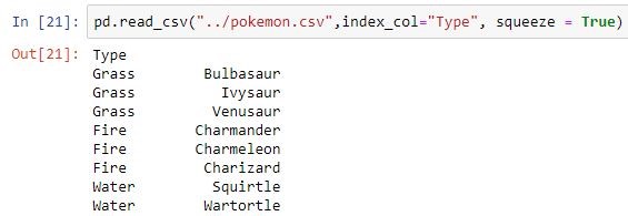
Makes passed column as index instead of 0, 1, 2, 3…r
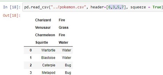
Makes passed row/s\[int/int list] as header
>>> df = pd.DataFrame({'animal': ['alligator', 'bee', 'falcon', 'lion',
>>>                   'monkey', 'parrot', 'shark', 'whale', 'zebra']})

>>> df.head()

      animal
0  alligator
1        bee
2     falcon
3       lion
4     monkey
>>> df = pd.DataFrame({'float': [1.0],
>>>                    'int': [1],
>>>                    'datetime': [pd.Timestamp('20180310')],
>>>                    'string': ['foo']}
>>> df.dtypes

float              float64
int                  int64
datetime    datetime64[ns]
string              object
dtype: object
>>> df.sort_values(by='col1', ascending=False, ignore_index=True)

  col1  col2  col3 col4
0    D     7     2    e
1    C     4     3    F
2    B     9     9    c
3    A     2     0    a
4    A     1     1    B
5  NaN     8     4    D
>>> df = pd.DataFrame({'key': ['K0', 'K1', 'K2', 'K3', 'K4', 'K5'],
>>>                    'A': ['A0', 'A1', 'A2', 'A3', 'A4', 'A5']})
>>>
>>> other = pd.DataFrame({'key': ['K0', 'K1', 'K2'],
>>>                       'B': ['B0', 'B1', 'B2']})
>>> df
  key   A
0  K0  A0
1  K1  A1
2  K2  A2
3  K3  A3
4  K4  A4
5  K5  A5

>>> other
  key   B
0  K0  B0
1  K1  B1
2  K2  B2

>>> df.join(other, lsuffix='_caller', rsuffix='_other')
  key_caller   A key_other    B
0         K0  A0        K0   B0
1         K1  A1        K1   B1
2         K2  A2        K2   B2
3         K3  A3       NaN  NaN
4         K4  A4       NaN  NaN
5         K5  A5       NaN  NaN
>>> df = pd.DataFrame({'Animal': ['Falcon', 'Falcon',
>>>                               'Parrot', 'Parrot'],
>>>                    'Max Speed': [380., 370., 24., 26.]})
>>> df

   Animal  Max Speed
0  Falcon      380.0
1  Falcon      370.0
2  Parrot       24.0
3  Parrot       26.0

>>> df.groupby(['Animal']).mean()
        Max Speed
Animal
Falcon      375.0
Parrot       25.0